A new perspective on Shapley values, part II: The Naïve Shapley method

** EDIT, Jan 2020: I renamed the method presented here Naive Shapley from the less intuitive Radical Shapley. This was changed throughout the post but the code snippets and git repository may still reflect the old name. **

Why should you read this post?

• For insight into Shapley values and the SHAP tool. Most other sources on these topics are explanations based on existing primary sources (e.g. academic papers and the SHAP documentation). This post is an attempt to gain some understanding through an empirical approach.
• To learn about an alternative approach to computing Shapley values, that under some (limited) circumstances may be preferable to SHAP (or wait for the next post for a more broadly-applicable idea).

If you are unfamiliar with Shaply values or SHAP, or want a short recap of how the SHAP explainers work, check out the previous post. In a hurry? I’ve emphasized the key sentences in bold to assist your speed-reading.

A more wordy introduction

My interest in Shapley values was sparked when I was using the SHAP library during a recent hackathon to explain the predictions of an Isolation Forest model. I noticed that for our model, the SHAP computation seemed to be quite inefficient, taking far too long to run on the entire dataset. So long, in fact, that I wondered whether in this case the “brute force”, exponentially-complex approach to Shapley values was actually a better option. This led me to write a function that computes Shapley values using an approach that seemed intuitive to me - instead of simulating missing features by integrating over their possible values (as in the SHAP method), they can be removed altogether from the model during training. For lack of an existing term in the literature I decided to refer to these as “Naive” Shapley values, in the sense that they are based only on the dataset (plus a model class) and not on a trained model.

One thing I learned as a neuroscience graduate student is that if you want to understand - and trust - your analysis tools, you need to subject them to careful empirical study as if they were your actual object of research. Reading the existing literature is important, as is getting hands-on experience yourself, but I find that real insight comes from not taking a tool’s results for granted but testing it in relation to artificial edge cases or other methods. The main idea of this post is then to better understand the advantages and limits of the SHAP explainers, by examining them in comparison to the Naive Shapley approach.

Code for the Shapley function and the examples used in this post is available here.

Outline (not quite a tl;dr)

In this post I will try to show the following:

• Naive Shapley values can be computed for a low number of features by retraining the model for each of 2^M feature subsets.
• The SHAP library explainers and the Naive Shapley method provide two different interpretations to Shapley values. The former is best suited for explaining individual predictions for a given (trained) model, and the latter better suited for explaining feature importance for a dataset and model class (e.g., a random forest, but not a specific trained random forest).
• Under some (limited) circumstances, the direct Shapley computation can be faster than the SHAP method. These circumstances are broadly when you a. have a low number of features (<~15), b. are using a model that is not supported by the efficient SHAP explainers and which has a relatively low training/prediction run time ratio (such as Isolation Forest), and c. need to compute Shapley values for a large number of samples (e.g., the entire dataset). In a future post I hope to eventually discuss a more practical polynomially-complex alternative of estimating Naive Shapley values with sampling.

So what are “Naive” Shapley values?

First, what is a Shapley value? If you have a team of people each contributing toward a total gain, but whose contributions are not necessarily independent (like a team manager’s contribution is dependent on also having contributing workers), then a Shapley value quantifies each one’s contribution to the total gain as the weighted average of their marginal contribution across all possible teams (so our team manager’s contribution might be 0 with no additional workers, 100 with at least one worker etc., and this is averaged across all possible permutations of the team). In more technical terms, a Shapley value reflects the expected value of the surplus payoff generated by adding a player to a coalition, across all possible coalitions that don’t include the player. 

In the realm of statistical models, Shapley values quantify the difference in the model’s prediction driven by adding each feature in the model. However, since such models typically cannot handle incomplete inputs, it’s not possible to simply remove a feature from the dataset in order to calculate its marginal contribution. Therefore, implementing the concept of Shapley values for explaining predictive models is matter of some interpretation. Specifically,

• the SHAP explainers interpret “adding a feature” in terms of it having a specific value vs. its value being unknown, for a given sample, during the prediction phase. For example, the marginal contribution of the “Age=30” to the output of a model predicting individuals’ income level can be computed relative to the mean predicted income level when substituting other possible values for “Age” from the dataset. On the other hand,
• the Naive Shapley method is based on the alternative intuition of measuring a feature’s impact in relation to it being absent from the model altogether during training. And so the contribution of “Age=30” in our example would be relative to the case of the model being initially trained with no Age feature at all.

Both interpretations are consistent with the mathematical notion of Shapley values, but they measure slightly different things.

Computing Naive Shapley values

The function for computing Naive Shapley values (code here) takes a dataset and a payoff function, computes the payoff for each possible feature combination (or, “player coalition”) and derives Shapley values according to the formula:

φ_i is the Shapley value for feature i, S is a coalition of features, v(S) is the payoff for this coalition, and N is the total number of features. N\{i} is all the possible feature coalitions not containing i. The first term within the sum corresponds to the fraction of times S appears within the possible feature permutations; intuitively, this gives the highest weight to the most informative contributions of a feature, i.e. when it is isolated or when it is added to a full set of features.

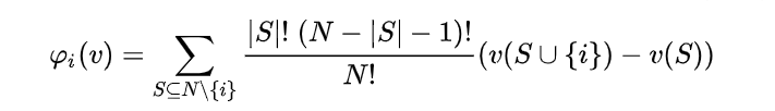
The output is the same format as that of the SHAP library explainers, and so all the SHAP plotting tools can be used to visualize it.

The payoff function can be any function that takes a dataset and returns a score (for instance, the profit generated by a team of workers). It is thus a general function that can be used for any kind of Shapley computation, but for the purpose of generating Naive Shapley values it will always be a function that trains a particular type of model on the dataset, and returns a prediction for each row.

For example: Let’s say we want to compute Naive Shapley values for an XGBoost model. We will write a custom payoff function that initializes an xgb model, trains it and returns a prediction for each sample (or perhaps only for a validation set). The Shapley function will feed the payoff function each possible combination of input features, and use the resulting outputs to compute a Shapley value for each sample and feature.

The main disadvantage of this algorithm is its computational complexity - it needs to run 2^M times (where M is the number of features), re-training the model each time. This complexity is of course the main reason the SHAP library was needed; on the other hand, under some limited circumstances this may be a faster option than using the SHAP Kernel explainer. The issue of comparative run time is covered at the end of this post.

How is this different from SHAP, and why should we care?

I compared results from the Naive Shapley method to both the SHAP KernelExplainer and TreeExplainer. I didn’t go into a comparison with the DeepExplainer, since neural network models rarely have the low number of input variables which would make the comparison relevant. As a quick summary, the Naive Shapley method differs conceptually from all SHAP explainers by representing features’ contribution to the model itself rather than to individual predictions; at the same time, it is generally slower (and impractical for more than a low number of features), although in some cases in may be more efficient than KernelExplainer. Once again, the previous post can help you if you’re not sure about what the SHAP explainers do.

Naive Shapley values vs. TreeExplainer

TreeExplainer is a good first candidate for the comparison with the Naive Shapley approach because unlike KernelExplainer they are both deterministic (not relying on sampling-based estimation) and insensitive to dependence between features (at least in TreeExplainer’s default implementation). This allows us to focus on the implications of the conceptual difference in how they treat missing features, namely, by re-training the model vs. integrating over feature values.

We can demonstrate the significance of this difference with a simple artificial example. Let’s generate a 3-feature linear regression model, with one feature x₁ which is a strong predictor of y, a second feature x₂ which is strongly correlated with it (and so slightly less predictive of y), and a third non-predictor feature x₃:

# Random dataset
num_samples = 10000
num_features = 3

X = pd.DataFrame(np.random.randn(num_samples, num_features)) # 3 random features
X[[1]] = X[[0]] + np.random.randn(num_samples,1)*0.2 # x2 is correlated with x1
y = X[[0]] + np.random.randn(num_samples,1) # y depends on x1 (and so also on x2) but not on x3
X.columns = ['Strong predictor of y', 'Correlated with strong predictor', 'Not a predictor of y']

To get Naive Shapley values, we need to first define the payoff function, which simply trains the model and returns its predictions (for simplicity I’m not including any training-validation split etc.).

import xgboost as xgb
def shapley_payoff_XGBreg(X,y):
    xgb_model = xgb.XGBRegressor(random_state=1) # if we don't fix the random state, Shaply values won't add up exactly to the final prediction.
    xgb_model.fit(X, y)
    out = xgb_model.predict(X)
    return out

And now run the Shapley function itself (reshape_shapley_output just re-arranges the original output, since compute_shapley_values returns a dictionary that does not assume a particular payoff format. An explanation of the function inputs and output is provided on github.

from radical_shapley_values import compute_shapley_values
from radical_shapley_values import reshape_shapley_output
mean_pred = np.mean(shapley_payoff_XGBreg(X,y))
radical_shapley_values = reshape_shapley_output(compute_shapley_values(shapley_payoff_XGBreg, X, y, zero_payoff = np.ones(ns)*mean_pred))

To get SHAP values, we’ll define the XGB regressor model, train it, and compute SHAP values with TreeExplainer:

import xgboost as xgb
import shap
xgb_model = xgb.XGBRegressor(random_state=1)
xgb_model.fit(X, y)
explainer = shap.TreeExplainer(xgb_model)
SHAP_values = explainer.shap_values(X)

Now let’s see how SHAP values and Naive Shapley values compare with each other. We’ll use the SHAP library’s neat summary_plot visualization tool, which plots the distribution of Shapley values for each feature:

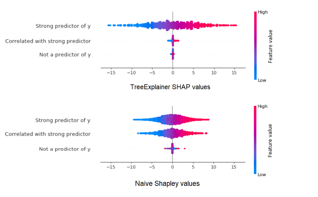
Let’s break this down:

• With the TreeExplainer, the model has already been trained with all 3 features, so SHAP values reflect the fact that x₁ has the highest impact within the trained model, while x₂ has a much smaller role as it is mostly redundant.
• With the Naive Shapley method on the other hand, x₂’s impact on y is almost as large as x₁’s because when the model is trained without x₁, x₂ is nearly just as informative.
• At the same time, the non-predictive x₃ is credited with a higher impact using the Naive Shapley method - simply because, especially as we did not do a training/validation split, it can over-fitted to the data in the absence of better predictors.

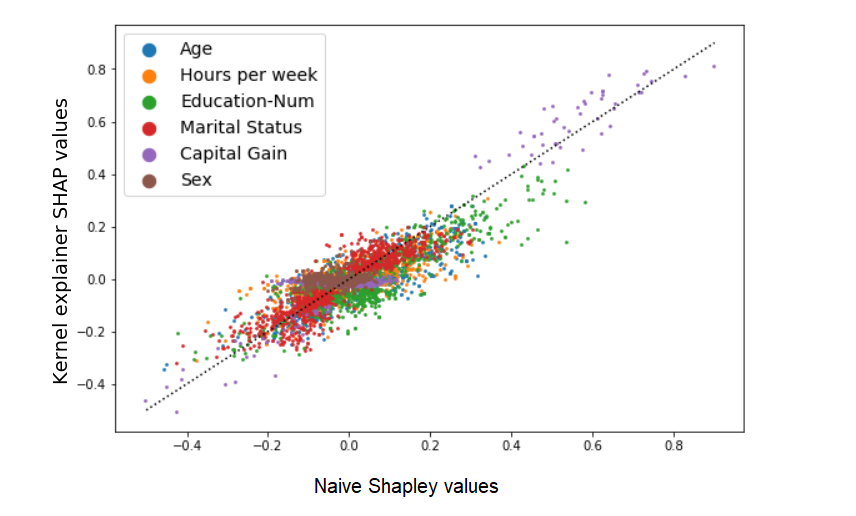
Now let’s try a real-world example. We will look at Shapley values for one of the datasets included in the SHAP library - the adult census database, with 12 demographic features that are used to predict whether an individual’s income is >50K$ (load with shap.datasets.adult()). For clarity and reduced computation runtime, we’ll include only 6 of the 12 features in our model (Age, Hours per week, Education, Marital status, Capital gain, and Sex). Our model will be an XGBoost classifier. How do the TreeExplainer SHAP values and Naive Shapley values compare with each other in this case? A scatter plot gives us a quick first impression:

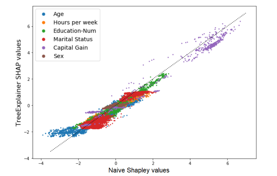
The results seem to be highly correlated, and this should already give us an indication that despite their conceptual differences, the two approach probably don’t diverge too drastically in their results. Now with summary_plot:

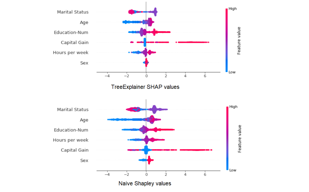
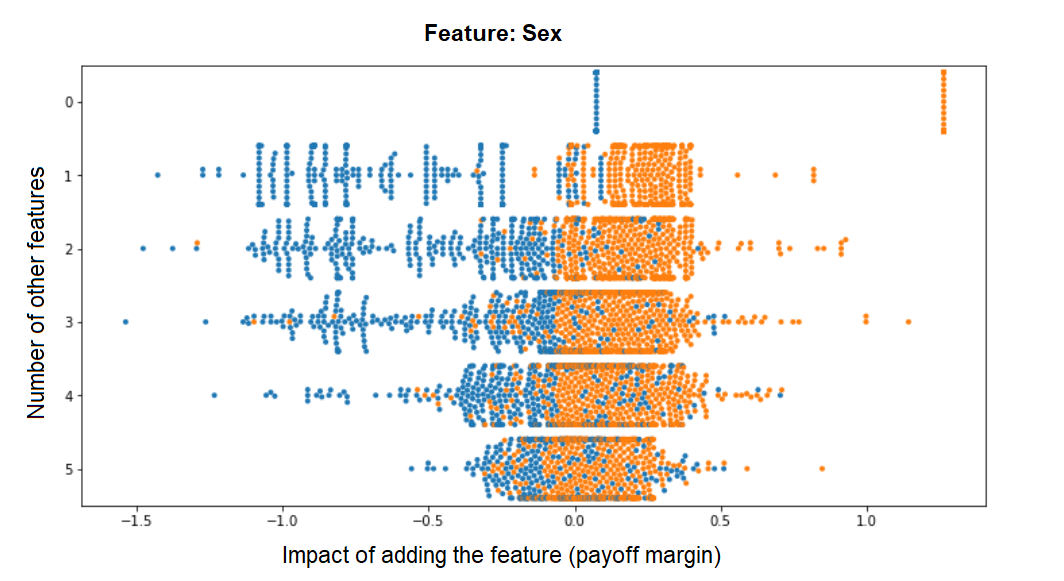
Here too the results seem similar enough (although different enough that the order of global feature importance is changed a bit). But let’s zoom in on the differences in how Shapley values for the Sex variable are distributed:

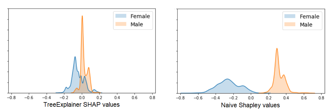
What’s going on here?

• The Naive Shapley results show us that averaged all possible feature combinations, adding this variable will have a consistent impact on prediction for this dataset (at least until we topple Patriarchy).
• The TreeExplainer results show us that in our trained model, this variable has a smaller and less consistent impact on prediction across our samples, most likely because it is used to explain smaller residual variance after most of the information it conveys was provided by other, more predictive features.

A benefit of implementing our own custom Shapley function is that we have easy access to a wealth of intermediate results - for example, the payoff margins that we calculated for each possible feature combination with vs. without a given feature (and whose weighted average is the Shapley value for each sample). Just for fun, I extracted it from the compute_shapley_values function so we can have a look at how the final Shapley values arise from these individual payoff margins. These are the distributions of payoff margins for the Sex variable, plotted against the number of features to which it is added:

Each point is the prediction difference for a single sample caused by adding the feature to a specific feature combination. Color corresponds to feature value levels (female/male). There were originally more points in the middle rows due to more possible feature combinations, which was mitigated by random sub-sampling.

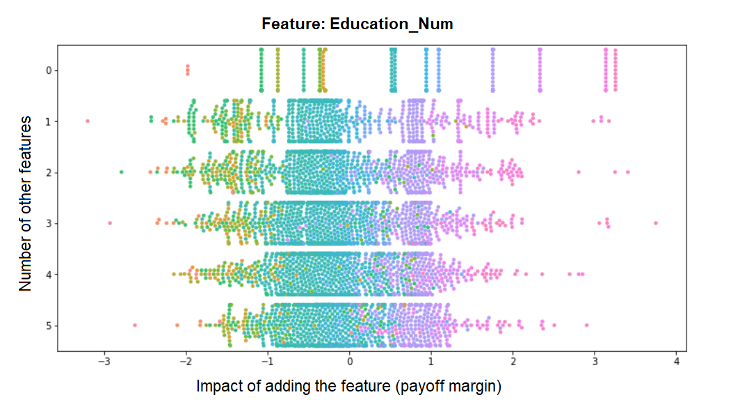
We can see how the more features are already in the model, the marginal impact of this feature becomes smaller and less bimodal (the bimodality we see in the previous histogram is therefore mostly driven by feature combinations from the upper rows). Contrast this to the distribution of margins for Education_Num for example, whose contribution remains pretty much fixed no matter how many other features make up the model - indicating that its contribution to the model is largely independent of them:

So - which method should we use to explain the role of the Sex variable in our data and model? I think the best way to put this is:

• Naive Shapley values better represent the global impact of the features in our dataset, while
• SHAP values better explain specific predictions given our existing trained model.

Two additional notes before moving on:

• A practical note: I am not suggesting that if you care about global feature impact in your dataset you should necessarily use the Naive Shapley method - mainly because in most cases that would be computationally intractable (although see the final sections for when it might not be). It is also apparent from my examples that the SHAP explainers’ results are typically not so different that they should not be used for this purpose. My main motivation here is to get a better understanding of SHAP results and their limitations.

• A technical note: If you are familiar with TreeExplainer, you may know that since in the case of binary classification the weights of the tree nodes hold not probabilities but log-odd values (which are transformed into probabilities with the logistic function as a final step) - the default optimization approach utilized by TreeExplainer provides SHAP values that add up to these untransformed values (and not the final probabilities). Simply applying the logistic function to the SHAP values themselves wouldn’t work, since the sum of the transformed values != the transformed value of the sum. To produce SHAP values that correspond directly to probability outputs, the TreeExplainer has to sacrifice some of its efficiency and use an approach similar to the KernelExplainer of simulating missing features by replacement with a background dataset - naturally a slower and less exact method. On the other hand, to directly explain probability outputs with the Naive Shapley method all that we need to do is choose the output of the payoff function to be the probability. Since with the Naive Shapley method we always pay the maximum computation cost, we might as well use a payoff function that gives us exactly what we want our Shapley values to explain.

Naive Shapley values vs. KernelExplainer

KernelExplainer is a model-blind method for computing SHAP values. As a very quick recap, it works by:

1. Sampling only a small subset of the possible feature permutations.
2. For each such permutation, simulating “missing features” by generating many bootstrapped samples where values of these features are replaced with values from a small “background dataset”, and averaging these samples’ predictions.

This means that in comparison to TreeExplainer, KernelExplainer is:

1. Slower - a large number of predictions needs to be computed for each explained instance in the dataset (since missing values are simulated by averaging over many possible values of the feature).
2. Non-deterministic - KernelExplainer’s SHAP values are estimated, with variance introduced both by the coalition sampling method and the background dataset selection.

How does this add up when comparing KernelExplainer SHAP values to Naive Shapley values? Let’s use the same 6-feature census dataset predicting a >500K$ income as a test case. This time, Following the example of this SHAP library notebook, we will use a KNN model to make this prediction and the KernelExplainer to provide Shapley values, which we can compare to Naive Shapley values:

# 1. Compute SHAP values:
import shap
from sklearn.neighbors import KNeighborsClassifier
num_samples_to_explain = 1000 # KernelExplainer is slow, so we'll do this for only 1000 samples.
knn = KNeighborsClassifier()
knn.fit(X, y)
f = lambda x: knn.predict_proba(x)[:,1] # Get the predicted probability that y=True
explainer = shap.KernelExplainer(f, X.iloc[0:100]) # The second argument is the "background" dataset; a size of 100 rows is gently encouraged by the code
kernel_shap = explainer.shap_values(X.iloc[0:num_samples])

# 2. Compute radical Shapley values:
def shapley_payoff_KNN(X, y):
    knn = KNeighborsClassifier()
    knn.fit(X, y)
    return knn.predict_proba(X)[:,1] # this returns the output probability for y=True

from radical_shapley_values import compute_shapley_values
from radical_shapley_values import reshape_shapley_output
mean_prediction = np.mean(shapley_payoff_KNN(X,y))
radical_shapley = reshape_shapley_output(compute_shapley_values(shapley_payoff_KNN, X, y, zero_payoff=np.ones(X.shape[0])*mean_prediction))
radical_shapley = radical_shapley[0:num_samples_to_explain] # compute_shapley_values returns Shaply values for all rows, so this is just to match the output of the kernel explainer.    

Comparing the results:

The two methods produce different but correlated results. Another way to summarize the differences is that if we sort and rank the Shapley values of each sample (from 1 to 6), the order would be different by about 0.75 ranks on average (e.g., in about 75% of the samples two adjacent features’ order is switched). Let’s remember that we are not looking at the relation between exact values and their noisy estimation: rather, Naive Shapley values are a deterministic measure of one thing, and the kernel SHAP values are an estimation of another (related) thing.

A final point to stress here, I think, is that despite all the sources of variance between the two methods, the results are still very similar overall, telling us that in many cases these methods can probably be used interchangeably assuming that the differences are not crucial for us.

Can Naive Shapley be faster than KernelExplainer?

As we’ve established, the Naive Shapely method needs to re-train the model and produce predictions 2^{num. features} times. This makes it impractical whenever the number of features is not low (let’s say, more than 15-20). But is it comparable to the SHAP explainers for a low number of features?

One thing to get out of the way is that the optimized SHAP explainers will always be faster than the Naive Shapley method, but the model-blind KernelExplainer can be very slow when explaining a large dataset. To get a better idea, let’s see what goes into the run time of the KernelExplainer vs the Naive Shapley method:

	In relation to…		The KernelExplainer run time is…		The Naive Shapley run time is…
	Number of features		fixed (aside from the impact on prediction time)		exponential
	Training time		fixed		linear
	Prediction time		linear (but computed ~200K times for each explained prediction)		linear
	Number of samples to explain		linear		fixed (aside from the impact on train/predict time)

The bold entries emphasize the weaknesses of each method. The Naive Shapley method is of course most vulnerable to increasing the number of features, and is also dependent on model training time, whereas KernelExplainer is not affected by these factors (although its prediction becomes more variable with increased number of features). The disadvantages of the KernelExplainer in terms of run time is that while it does not need to spend time re-training the model, it runs separately for each explained prediction (while Naive Shapley runs for all predictions at once), each time having to produce predictions for ~200K samples (nsamples X num. background samples, which by default are 2048+2M and 100, respectively).

A good example for a model for which the Naive Shapley method can perform faster than KernelExplainer, for a low number of features, is an Isolation Forest model, a popular tool for anomaly detection, as despite being a tree-based model it is not supported by TreeExplainer and its training time (compared to prediction) is relatively fast. To demonstrate this, I am using the Credit Card Fraud Detection dataset from Kaggle, a ~285K sample, 30 features dataset used to predict anomalous credit card transaction. For our demonstration let’s use 100K samples and reduce the 30 features down to 15. On my old laptop I get the following approximate run times:
Train the model: 8 sec
Make predictions for all 100K samples: 8 sec
Compute SHAP values for a single prediction: 18 sec (which is, unsurprisingly, about the time it takes to compute predictions for ~200K bootstrapped samples)

Based on this we can make a rough estimate of how long it would take to compute Shapley values for the entire dataset. The KernelExplainer should simply take 100,000 x 18 seconds, or about 500 hours. The Naive Shapley function will run for up to 2¹⁵*(15+13) seconds, or about 150 hours (actually, a better estimate may be about 50 hours since the bootstrapped datasets used for training in each iteration of the algorithm will have between 1 to 15 features, or 7–8 on average, making training typically faster). Both methods are slow (though both could benefit from parallelization), but what’s important here is not the specific example but understanding where the computation time comes from in each case. To summarize:

• If you need to explain only a small group of “important” predictions, KernelExplainer should be fast enough.
• If you need to explain a million predictions and you have less than 10-15 features, the Naive Shapley method should be much faster.

A practical compromise? Estimating Naive Shapley values with sampling

(This part is basically a teaser for the next post).

What if our model is only supported by KernelExplainer, and we really need Shapley values for our entire huge dataset - but there are too many features to compute Naive Shapley values?

Well, why not try to estimate Naive Shapley values using coalition sampling? Using random sampling to estimate Shapley values for a high number of players (as is done e.g. by the KernelExplainer) has been thoroughly discussed in the literature and improved methods are still being developed (see for example Castro et al. 2009, Castro et al. 2017 or Benati et al. 2019). I would suggest that sampling can work well in combination with the Naive Shapley approach - that is, to sample the space of feature combinations on which the model is trained (thus not needing to simulate missing features by averaging over bootstrapped samples).

Getting rid of the exponential component in the algorithm would drastically reduce run time and make the approach feasible for a high number of features (at the expense of some estimation variance), while keeping the re-training approach would still ensure a short run time when computing Shapley values for large datasets.   This is only a theoretical idea, and I would not make this post longer than it already is by developing it further. I would however be happy to get any comments you may about this (maybe you’ve already encountered this idea somewhere else?), and I hope to get a chance to complete this project and discuss it in a future post.

If you wish to comment on this post you may do so on Medium.